This application is a web-based neural network training interface that allows users to train a neural network on
the fly within their browser using TensorFlow.js. It's particularly useful for educational purposes, to
visualize how different parameters affect the learning process, and for rapid prototyping of simple neural
network models.
Here's a breakdown of the different controls and how they could be used:
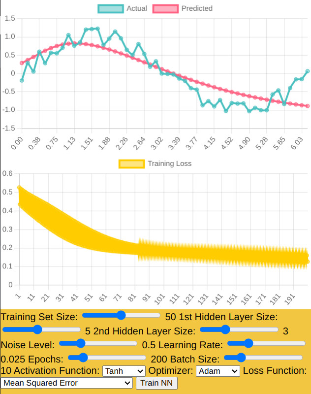
Training Set Size: This slider adjusts the number of data points used to train the neural
network. A larger dataset can potentially improve the model's accuracy but may take longer to train.
Hidden Layer Size: These sliders control the number of neurons in the first and second
hidden layers of the neural network. More neurons can capture more complex relationships in the data but
also increase the risk of overfitting and require more computational resources.
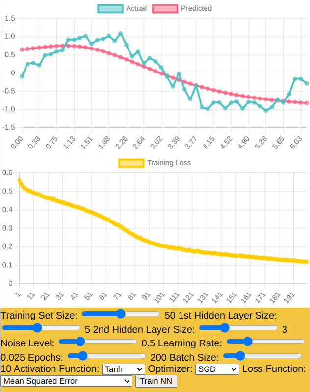
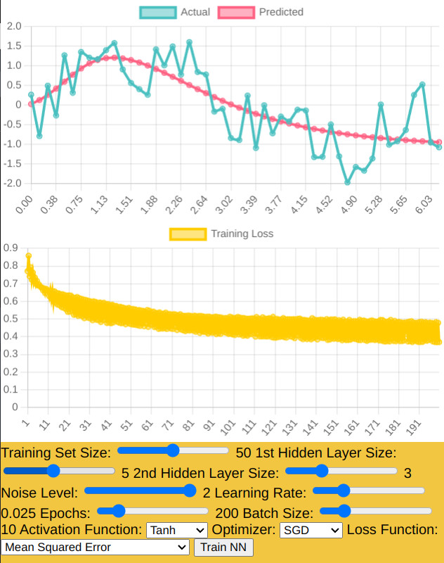
Noise Level: This slider adds a certain level of randomness to the training data,
simulating real-world data imperfections. It helps to test the robustness of the neural network against
noisy data.
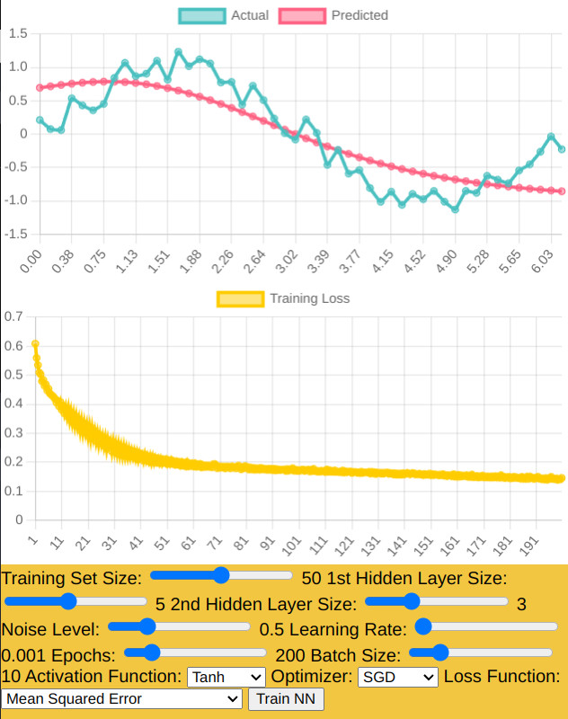
Learning Rate: This is a critical hyperparameter that affects how quickly the model learns.
Too high a learning rate can cause the model to converge too quickly to a suboptimal solution, while too low
a rate can slow down the training process significantly.
Epochs: This slider sets the number of times the learning algorithm will work through the
entire training dataset. More epochs can lead to a more trained network, but also increase the risk of
overfitting if too many are used.
Batch Size: This determines the number of samples that will be propagated through the
network before updating the model parameters. Smaller batch sizes generally require less memory and can
update the model more frequently.
Activation Function: This dropdown lets the user choose the activation function for the
hidden layers. Options like ReLU, Sigmoid, and Tanh dictate how the neurons in the network will transform
the input signal into an output signal.
Optimizer: This dropdown allows the selection of the optimization algorithm that will
minimize the loss function. Choices like Adam, SGD, and Adagrad offer different approaches to the learning
process.
Loss Function: Through this dropdown, the user can choose the loss function the model will
use to compute the quantity that a model should seek to minimize during training. Options include Mean
Squared Error, Mean Absolute Error, and Mean Squared Logarithmic Error.
Train NN Button: When clicked, this button starts the training process with the selected
parameters. It’s the action trigger for the model to start learning from the data.
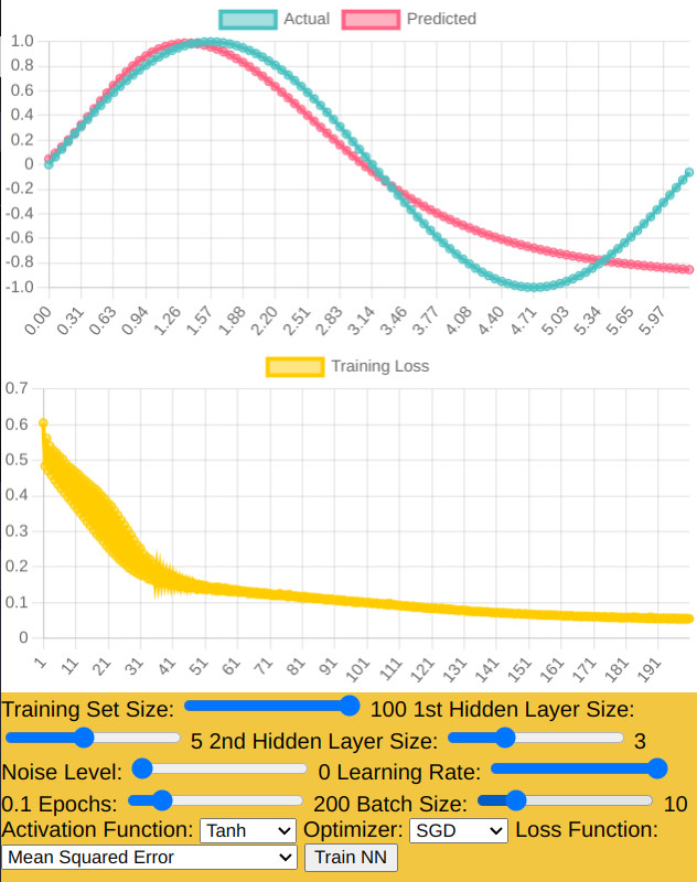
The two charts display in real-time the performance of the neural network:
Prediction Chart: Shows the actual data points versus the predictions made by the neural
network.
Training Loss Chart: Illustrates the model's loss over each epoch, providing insight into
how well the training process is going.
Overall, the application can serve as a didactic tool for understanding neural networks and a practical
instrument for researchers and hobbyists interested in experimenting with machine learning without needing to
set up a full-fledged environment.
Understanding Fluctuations in Neural Network Loss During Training
If you're observing fluctuations or jumps in the loss, especially if the loss increases sharply at certain
points, this could be due to several factors:
Learning Rate: If the learning rate is too high, the model may overshoot the minimum of the loss function.
The learning rate of 0.04 could be too high, causing instability in the training process.
Batch Size: A batch size that's not appropriate for the dataset might cause erratic updates to the weights,
leading to fluctuations in the loss.
Optimizer: Although Adam is robust, it might still require tuning of its parameters (like learning rate
schedules, or beta values) to stabilize the loss.
Data Quality: Make sure the data is clean and preprocessed correctly. Anomalies or outliers can cause sudden
changes in loss.
Model Complexity: Ensure that the model is appropriate for the task. Both underfitting and overfitting can
cause erratic loss patterns during training.
Randomness: Stochastic processes in training can cause variability. This includes the random initialization
of weights, random shuffling of the dataset, and randomness in dropout layers (if used).
Loss Calculation: Ensure the loss is averaged correctly over batches and epochs. Summing losses without
averaging can cause misleading spikes.
To reduce the fluctuation:
Try a smaller learning rate or use learning rate schedules to decrease it over time.
Consider tuning the batch size, starting with smaller batches and increasing if needed.
Introduce techniques like gradient clipping to limit the effect of very large gradients.
Implement early stopping to halt training when the validation loss starts to rise, which can prevent
overfitting and reduce the likelihood of these spikes.
Use a more complex model evaluation approach. Instead of just looking at loss, also look at validation
metrics. Loss might not tell the full story, especially if the distribution of errors is skewed.
Remember that manually fine-tuning hyperparameters can be quite tedious. You might want to implement a more
systematic approach, like a grid search, random search, or even more advanced methods like Bayesian
optimization, to find the optimal set of hyperparameters.
When training neural networks, especially when using stochastic algorithms like SGD (Stochastic Gradient
Descent) or its variants (like Adam), it's expected to get different results across runs even with the same
initial parameters. This is due to the inherent randomness in the training process, including but not limited
to:
Random Initialization: Neural networks typically start with randomly initialized weights. Even slight
differences in these starting values can lead to different training paths and results.
Data Shuffling: If the training data is shuffled before each epoch (which is common practice), the order of
data seen by the network changes, which can affect the updates to the model.
Stochastic Gradient Descent: The optimizer itself is stochastic. Adam, for instance, calculates adaptive
learning rates for different parameters from estimates of first and second moments of the gradients; the
stochasticity in the gradients will lead to different updates.
Hardware: The computation may involve floating-point arithmetic, where operations can be non-associative due
to rounding errors, leading to small variances.
Parallelism and Concurrency: The way computations are parallelized on the CPU/GPU can also introduce
non-determinism.
Improving Neural Network Performance for Sinusoidal Function Prediction
For a neural network model tasked with learning a sinusoidal function without noise, achieving a near-perfect
prediction is feasible, especially if the network architecture, learning rate, and other hyperparameters are
suitably chosen. Here are some suggestions to fine-tune your existing setup to improve model performance:
Simplify the Model: Since the task is to predict a sinusoid, a simple model should suffice.
You might not need two hidden layers. Try with one hidden layer first, and only add a second one if
necessary.
Hidden Layer Neurons: You may not need as many neurons. Try starting with a smaller number
and increase only if the model performance is not satisfactory.
Learning Rate: The learning rate may be too high, leading to overshooting the minimum loss.
You should consider lowering it or using a learning rate schedule to decrease it as training progresses.
Activation Function: The choice of ReLU (Rectified Linear Unit) is fine for hidden layers
in many cases, but since the sinusoidal function involves both positive and negative values, `tanh` might be
a more suitable choice as it outputs values in the range [-1, 1].
Loss Function: Mean Squared Error (MSE) is appropriate for regression problems, and since
you're predicting a continuous value, it's a suitable choice.
Epochs and Batch Size: Your choice of 200 epochs and a batch size of 10 seems reasonable,
but these may need to be adjusted based on the model's learning curve.
Optimizer: Adam is generally a good optimizer, but if you find the loss fluctuating too
much, you might want to try SGD with momentum or experiment with different hyperparameters for Adam.
Randomness: TensorFlow.js, like many deep learning libraries, includes randomness in weight
initialization and data shuffling. While you can't set a global seed, try to ensure consistency in other
ways such as data preprocessing and model initialization.
Regularization: If you have a larger model or add noise later, you may need regularization
techniques like dropout or L1/L2 regularization to prevent overfitting.
Data Normalization: Make sure the input data is normalized or standardized if you start
working with more complex or varied datasets.
Evaluate on Unseen Data: Ensure that you're evaluating model performance on a separate test
set that the model hasn't seen during training to get a true measure of its predictive power.
Experiment Systematically: Change one hyperparameter at a time to see its effect on the
model's performance. This can help you understand which parameters are most sensitive and need careful
tuning.
Based on these suggestions, you can adjust your training script to conduct more systematic experiments and
converge on an optimal set of parameters that yields the best performance for your sinusoidal prediction task.